EMPIAR-10673 Tutorial
Calculating a 3.2 angstrom map of a GPCR membrane protein in under 2h
- Time requirement: 1.5 h compute time | 20- 40 min manual time | 9 jobs
- Goal: Determine a 3.2 angstrom structure of GLP1R.
- Data: available upon request.
This tutorial will walk you through the analysis of the EMPIAR dataset 10673 containing GLP1R.
Creating a Project
To start, you need to create a new project. Navigate to the Project view by clicking on the Project tab in the left sidebar. To Create a new Project, click on the top right button "+Add new project". Enter a name and specify the type (SPA for this tutorial).
Once you confirm, the project grid will open automatically.
Linking a dataset
To run any type of analysis in a CryoCloud project, you need to link a dataset to your project.
Click on the "Datasets" tab on the top left, and select the dataset of Empiar-10673.
Pre-processing
This section focuses on the jobs you can run in the pre-processing column.
Motion Correction
To set up a motion correction, click on the "+" tile in the Pre-processing column. The job type (Motion Correction) and the linked dataset will already be pre-selected in the dropdowns, so you just need to confirm the selection.
Once confirmed, the Job setup form will open. The movies.star will be already pre-selected as it was created for the linked Empiar dataset during upload - there is no need to run a separate Import Job on CryoCloud, as the .star files will be automatically created during dataset upload.
Specfy the following parameters
Input movies STAR:datasets/<N>/movies.stargain reference:datasets/<N>/gainref.mrc
After that, confirm the setup and submit the job by clicking "Save & Run" on the bottom right. The job status will change to submitted, and analysis will start in 3-5 min, during which an instance is spun up for you. The Motion Correction job itself should finish in about 18 min.
CTF Estimation
You can queue a job to a running job or a job draft. Simply click on the "+" sign on the top right of a job tile. After setting up and submitting the job, its status will be shown as queued and it will automatically start when the previous job has finished.
After submitting the MotionCor job, you can go back to the overview and set up the next CTF Estimation job - there is no need to wait for the previous job to be finished, as you can queue the CTF Estimation job to the running MotionCor job.
Simply click on the "+" in the top right corner of the MotionCor Job, select CTF Estimation/Find job with the MotionCor job as a parent, and specify all parameters in the job view. For this job, you can keep all default parameters - so if you like simply jump to the bottom and click "Save & Run".
The Job should finish in about 2 minutes and show you a plot of your major results as well as large micrograph previes on your right.
Micrograph Selection
Next, we want to exclude micrographs with a resolution lower than 3.5 Å, as done in the publication by Danev et al.
Set the upper slider of the CTF max reoslution plot to 3.5 and click selection on the top right of the plots. This will create and open a new Interactive Select job. Run it by clicking 'Run' on the bottom right.
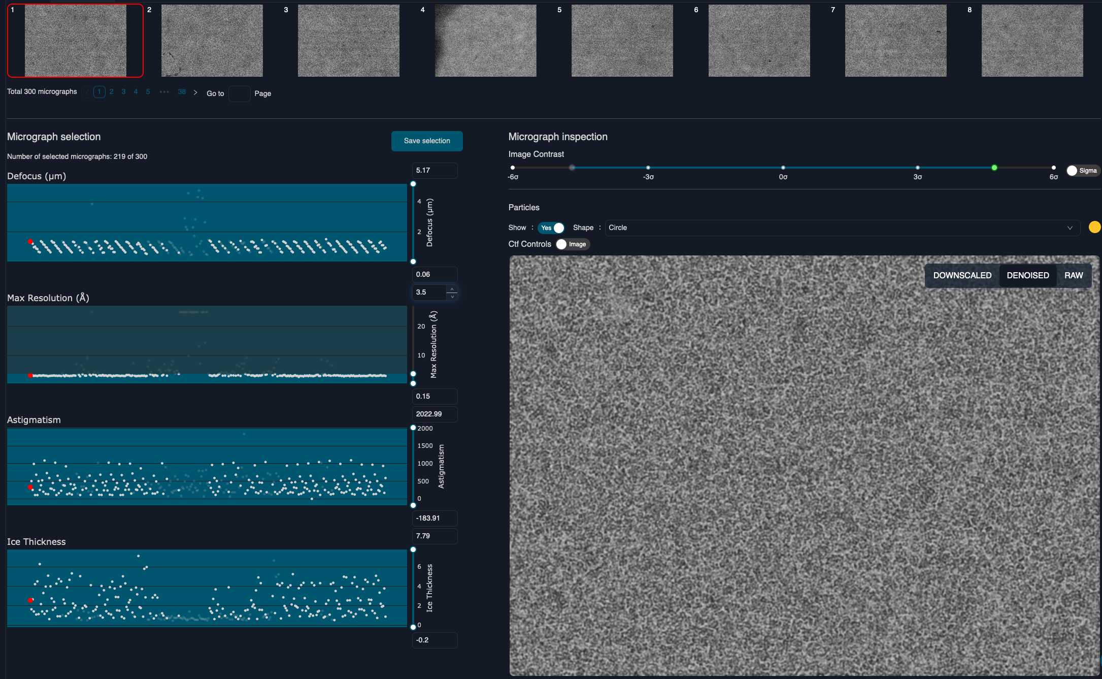
This results in 219 selected micrographs.
Particle Picking
Set up a particle picking job, either as before by clicking on the "+" of the CTF job, or by hovering over the Pre-Processing column, clicking the "+" sign and specifying the CTF job as input. For this dataset, you can use the default values with the LoG picker. You just need to specify the minimum and maximum diameter as 100 angstrom and 160 angstrom respectively:
Min. diameter for LoG filter (A):100Max. diameter for LoG filter (A):160
Just like for the CTF job, you can inspect the results of your picking job once it's finished in the results section. The picking should have resulted in about 179k particles.
Extract Particles
To analyze your picked particles you need to extract them first. Set up an Extract Particle job via the "+" sign on the Picking job tile.
If you struggle finding a job from the list of available jobs, you can type in the first letters and the list will be automatically filtered accordingly. You can try this by typing in the first letter of the 'Extract Particles' job.
After creating the job, specify the following parameters:
Micrograph STAR file:jobs/InteractiveSelect/<N>/micrographs_ctf.star(from Interactive Select job)Input coordinates:jobs/AutoPick/<N>/coords_suffix_autopick.star(from AutoPick job)Particle box size (pix):256Rescale particles:YesRescaled box size (pix):70
You can keep the default values for the other settings and submit the job.
Class3D
This section focuses on the jobs you can run in the Class3D column.
Uploading a reference map
Before we go to the 3D classification step, you need to upload a reference map to your project.
In CryoCloud, all references, masks and other auxiliary files can be uploaded to the Project's Archive located next to Datasets on the top left.
You can use these files as input for jobs that require external data (masks, references, high resolution maps for model building).
Simply click on the "Archive" button. This will open a Side Panel that allows you to upload new files and inspect all current files in the Archive. You can download the following reference and mask and upload it to the project's archive by clicking on "Upload file" on the Side Panel:
Instead of using the provided mask, you can also create one on after your 3D classification job from your selected class. Simply add a Mask Create job on top of your Class3D job
3D Classification
For this dataset, we will go directly to the 3D classification step as was done by the authors.
Create a Class 3D job and specify the following parameters:
Input images STAR file:jobs/Extract/<N>/particles.star, whereNis the previous job's number and is set automatically.Reference map:archive/<downloaded-reference>.mrcInitial low-pass filter:20Number of classes:3Mask diameter (A):160Use fast subsets (for large datasets)?:NoUse Blush regularization:Yes
All other parameters can be kept at their default values. The 3D classification job should finish in about 50 minutes.
Selecting good classes
Once the 3D classification job is finished, set up a Select job on top of the previous job tile Class 3D.
As the job's input, select the last iteration from the parent job, it should look like this:
Select classes from model.star:jobs/Class3D/<N>/run_it<X>_model.star, whereNis previous job's number andXis the last iteration (in the previous step we set it to 25)
Click "Load selector" to load the 3D class averages. You can then interactively select the correct classes (shown below).
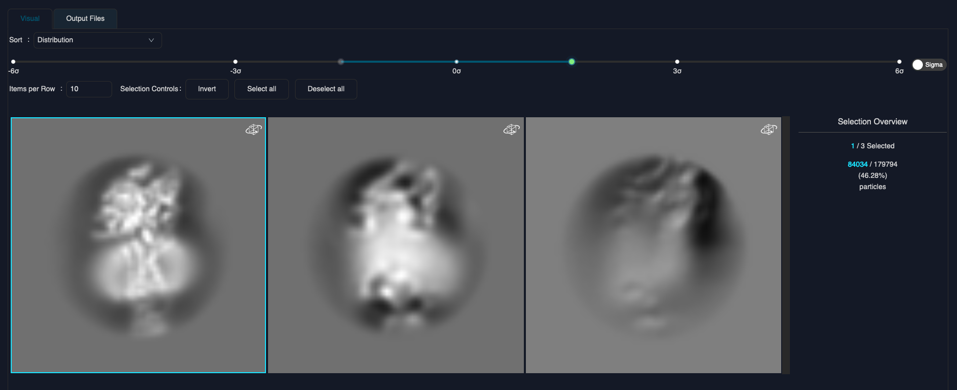
Once you selected all classes, click the "Save & Run" at the bottom to submit the job. This should extract about 85k particles.
Extract Particles
Next, we want to extract particles with a larger box and smaller pixel size in order to obtain a higher resolution with the subsequent 3D refinement job.
Setup an Extract Particles job with the following settings:
Micrograph STAR file:jobs/Select/<N>/micrographs_ctf.star(from InteractiveSelect job)OR re-extract refined particles:YesRefined particles STAR file:jobs/AutoPick/<N>/coords_suffix_autopick.star(from select job)Particle box size (pix):256Rescale particles:YesRescaled box size (pix):140
This job will take approximately 2 min.
Refine3D
3D Refinement
After submitting your Extract Particles Job, setup your Refine3d job.
Use the selected particles from the Class 3D job and the uploaded reference in the archive as input for the Refine 3D job:
Input images STAR file:jobs/Select/<N>/particles.starReference map:archive/<downloaded-reference.mrc>Mask:archive/<downloaded-mask.mrc>
Additionally, you need to specify the following parameters:
Initial low-pass filter:10Mask Diameter (A):160Use solvent-flattened FSCs:YesUse Blush regularization:YesUse finer angular sampling faster:Yes
You can keep all other settings as default, and submit the job which should finish in about 30 minutes and result in a map at 3.2 A resolution.
Next Steps: Sharpening, Model building & Visualization
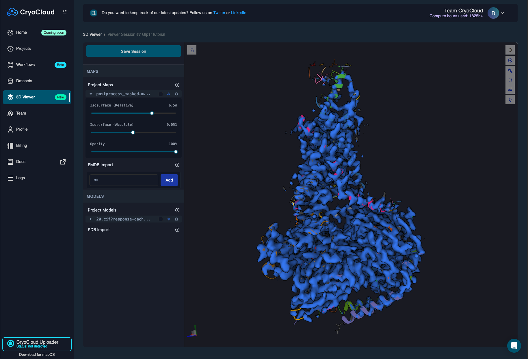
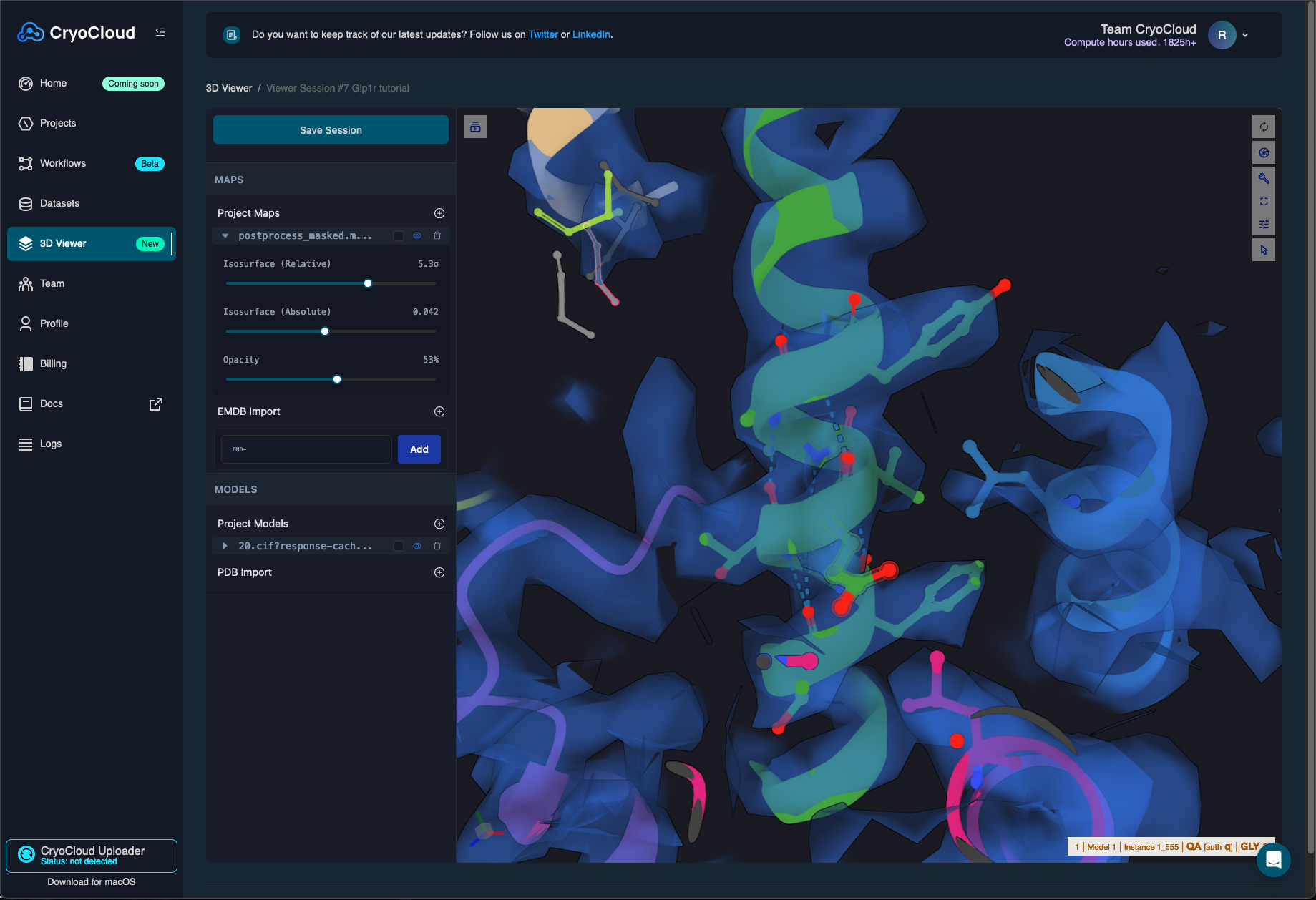
Now that you have a high resolution map of GLP1R, you can run a ModelAngelo to build an intial starting Model into the map. Prior to creating a ModelAngelo job, make sure to run a postprocessing job to sharpen your map and use that as input for ModeAngelo. Both jobs should finish in about 3min.
You can load both your sharpened map and the newly build model in a new 3D viewer session which will look as follows:
You can also run polishing and CTF refinement jobs with the available data.
If you have any input or questions during the tutorial, let us know via the in-app messenger or an email to hi@cryocloud.io.
If you have read through the tutorial but not signed up for a free 30-day CryoCloud trial, you can do that here.